import skrf as rf
import numpy as np
# pyright: reportCallIssue=false

Measurement Extraction

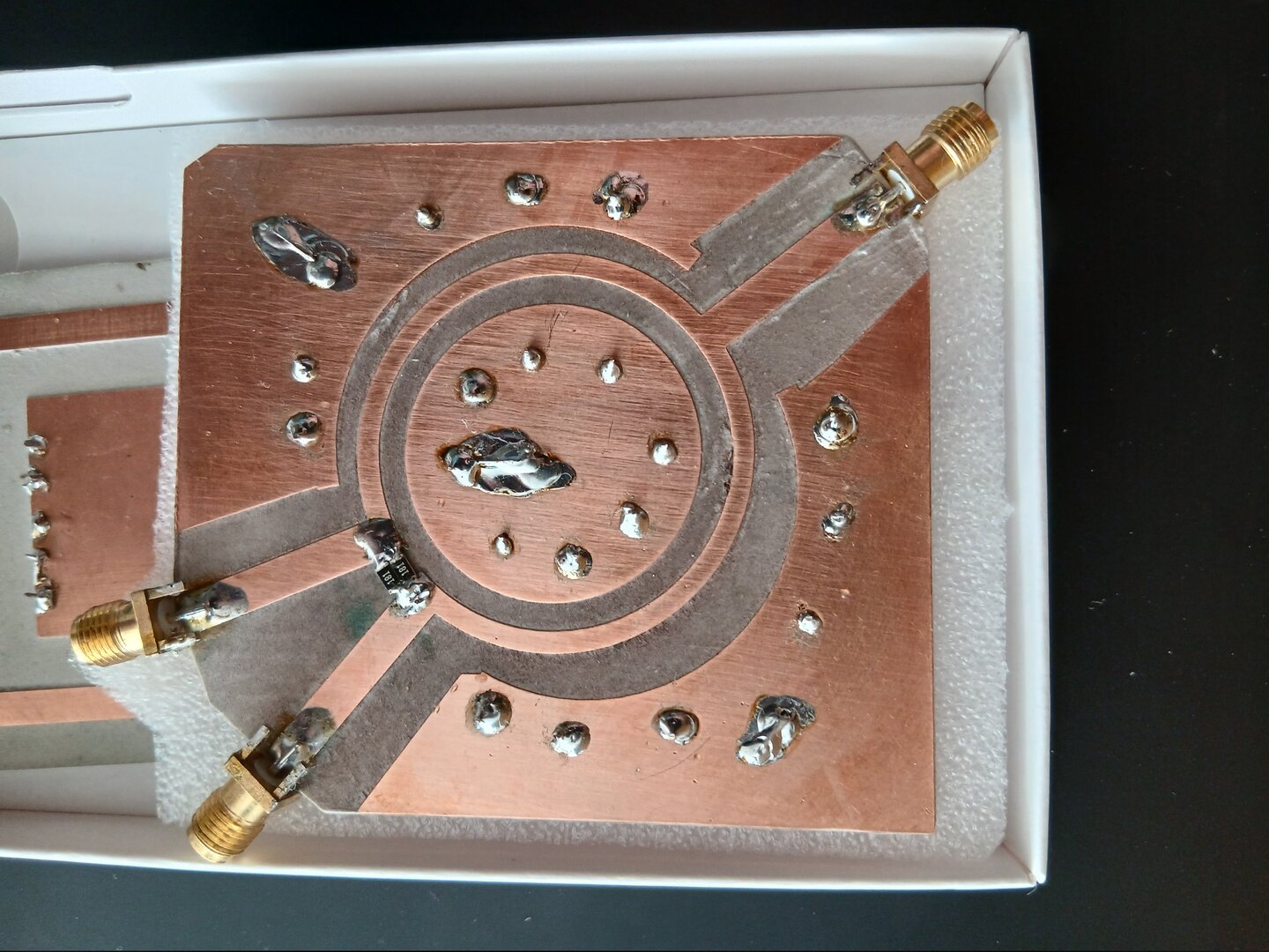
For physical measurements, a 2-port Rohde-Schwarz ZNC3-2Port VNA was used, calibrated in a frequency range from $0.5$ to $1.5$ GHz. Since the Wilkinson divider has 3 ports, the S-parameter matrix is reconstructed through 3 separate measurements.

The VNA port -> Wilkinson port correspondence is:

File	VNA Port	Device Port
1.s2p	1	2
1.s2p	2	3
2.s2p	1	1
2.s2p	2	2
3.s2p	1	1
3.s2p	2	3

Finally, we have another file 4.s2p, which contains the through connection between the two cables without any load in between to see the inherent ripple of the instrument/cables

First, we load the four measurement files

m1 = rf.Network('mediciones/1.s2p')
m2 = rf.Network('mediciones/2.s2p')
m3 = rf.Network('mediciones/3.s2p')
m4 = rf.Network('mediciones/4.s2p')

Then we create a three-port network corresponding to the Wilkinson divider called wilkinson

# Extract frequencies from the first file
freq = m1.frequency
# Generate zero matrix to initialize empty network
s_mat = np.zeros((len(freq), 3, 3), dtype=complex)
# Generate empty network
wilkinson = rf.Network(frequency=freq, s=s_mat, z0=50, name='Wilkinson 3-port')

The notation to refer to an S-parameter is wilkinson.s[freq, Sa, Sb]. To operate over all frequencies, simply work in full-range mode using wilkinson.s[:, Sa, Sb]. Indexing starts at 0, not 1, so to refer to, for example, the $S_{21}$ parameter across the entire available frequency spectrum, use wilkinson.s[:, 1, 0]

Now we will map all parameters stored in the .s2p files (each corresponding to a two-port network specified in the table) to the three-port network wilkinson corresponding to our power divider.

For transmission measurements, there is only one option in each case, so we simply map from the s2p file to the variable

# File 1.s2p (m1): VNA p1 -> Device p2 | VNA p2 -> Device p3
wilkinson.s[:, 2, 1] = m1.s[:, 1, 0]  # S21 from m1 -> S32 of device (transmission p2->p3)
wilkinson.s[:, 1, 2] = m1.s[:, 0, 1]  # S12 from m1 -> S23 of device (transmission p3->p2)

# File 2.s2p (m2): VNA p1 -> Device p1 | VNA p2 -> Device p2
wilkinson.s[:, 1, 0] = m2.s[:, 1, 0]  # S21 from m2 -> S21 of device (transmission p1->p2)
wilkinson.s[:, 0, 1] = m2.s[:, 0, 1]  # S12 from m2 -> S12 of device (transmission p2->p1)

# File 3.s2p (m3): VNA p1 -> Device p1 | VNA p2 -> Device p3
wilkinson.s[:, 2, 0] = m3.s[:, 1, 0]  # S21 from m3 -> S31 of device (transmission p1->p3)
wilkinson.s[:, 0, 2] = m3.s[:, 0, 1]  # S12 from m3 -> S13 of device (transmission p3->p1)

Now the reflections. There are 2 measurements of each since each port was used in two different files. Without information about which is more reliable, we take a simple average of all reflections

# Reflection S11 (average of m2 and m3)
aux = (m2.s[:, 0, 0] + m3.s[:, 0, 0]) / 2  # Average of S11 from m2 and S11 from m3
wilkinson.s[:, 0, 0] = aux  # S11 of device

# Reflection S22 (average of m1 and m2)
aux = (m1.s[:, 0, 0] + m2.s[:, 1, 1]) / 2  # S11 from m1 -> S22, S22 from m2 -> S22
wilkinson.s[:, 1, 1] = aux  # S22 of device

# Reflection S33 (average of m1 and m3)
aux = (m1.s[:, 1, 1] + m3.s[:, 1, 1]) / 2  # S22 from m1 -> S33, S22 from m3 -> S33
wilkinson.s[:, 2, 2] = aux  # S33 of device

Now the wilkinson block has the complete S-parameter matrix extracted through measurements.

Plots

We plot transfer, matching, and isolation in three separate graphs using the plot_s_parameters function made separately to simplify and standardize plotting

We have three networks:

The first network is an ideal simulation made in ADS:

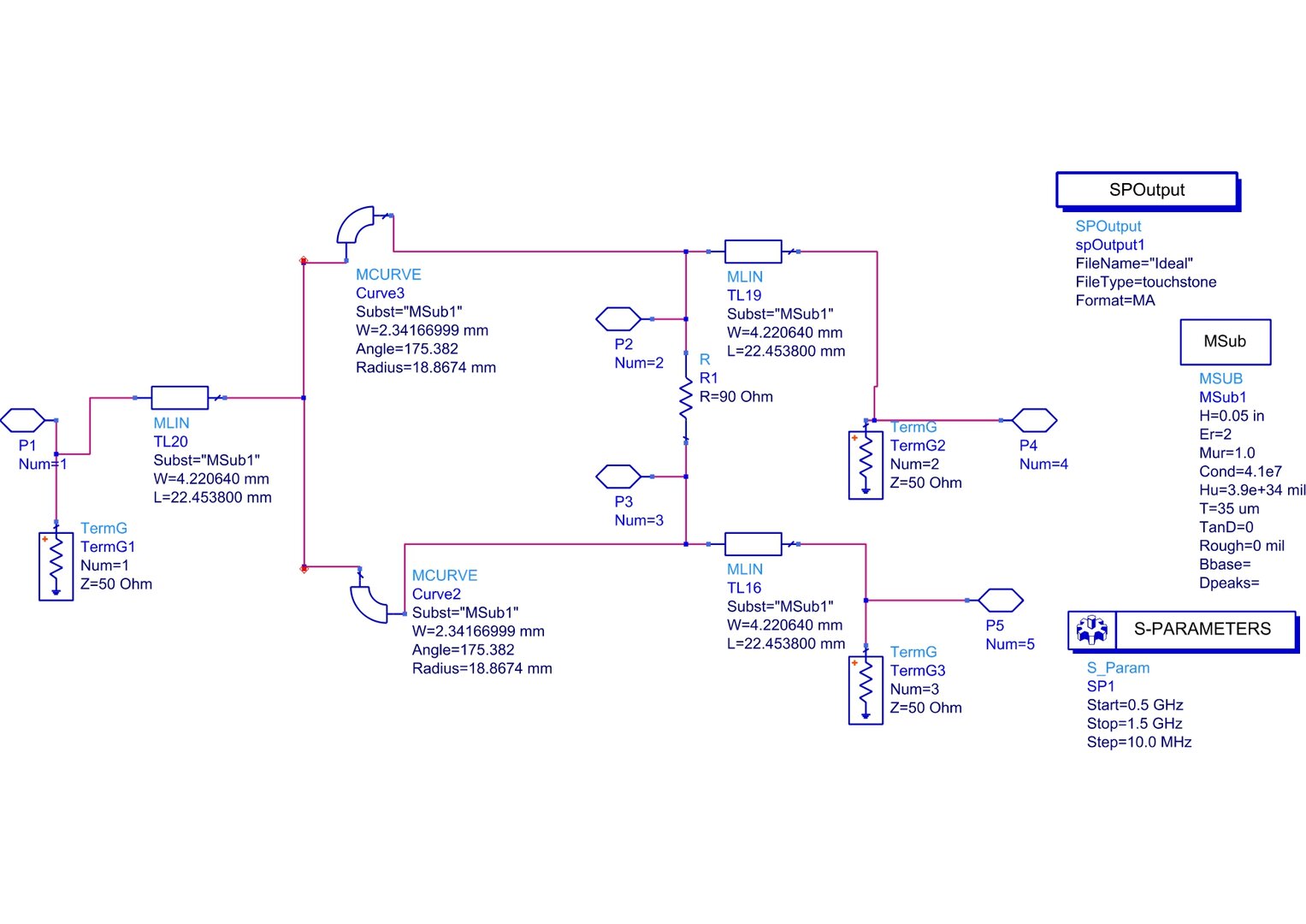
I import that network and call it wilkinson_ideal

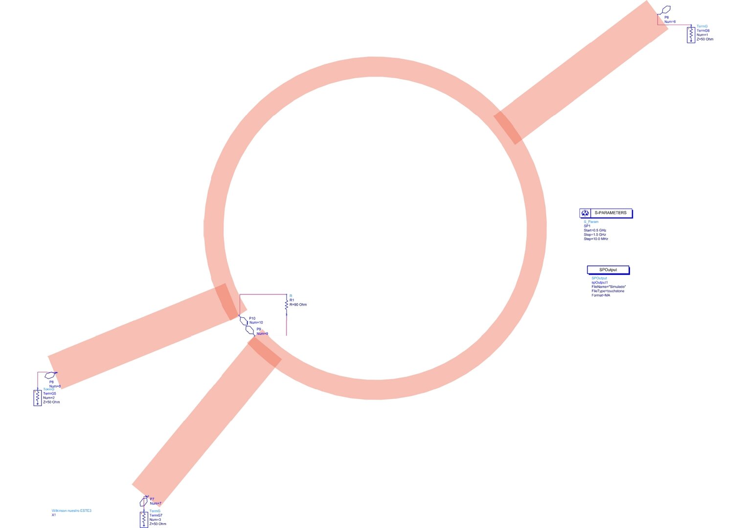
Then there's the simulation made in ADS where the physical block was simulated with substrate parameters and real resistors. I call that network wilkinson_simulado

And finally, the real measurements extracted from the VNA that we've been working with so far, which we rename to wilkinson_real

Since the simulations are exported as s3p parameters, i.e., 3-port network, not much processing is needed

# Prepare the three networks
wilkinson_ideal = rf.Network('simulaciones/ideal.s3p')
wilkinson_simulado = rf.Network('simulaciones/simulado.s3p')
wilkinson_real = wilkinson

from importlib import reload
import plotear  # Import the module (not the function directly)

reload(plotear)  # Reload the module from disk
from plotear import plot_s_parameters  # Re-import the updated function

Plotting function

Function saved in a separate file called plotear.py that plots with a standardized format for this case. The solid blue vertical lines are fixed at $1\text{GHz}$ while the dashed lines are the peaks (maximum or minimum as appropriate) of each curve. The value in $\text{GHz}$ of each dashed line is in the legend

First, plot the ideal one

plot_s_parameters(wilkinson_ideal, 'Ideal network analysis', save_fig=True, autoscales=True)

Then plot the parameters from the simulation

plot_s_parameters(wilkinson_simulado, 'Simulated network analysis', save_fig=True, autoscales=True)

And finally from the measured parameters

plot_s_parameters(wilkinson_real, 'Real network analysis', save_fig=True, autoscales=False)

Apart from the marked ripple, it can be seen that the trends are maintained regarding the peaks next to the phase shift

Instrument Error Correction

We also captured the .s2p parameters of a direct connection between the cables to see the ripple of our setup

through = rf.Network(frequency = m4.frequency, s = m4.s, z0=50, name='Through')

through.plot_s_db()

There is a huge difference between the transfers and the reflections. Focusing on the transfers

through.plot_s_db(m=1, n=0)
through.plot_s_db(m=0, n=1)

Aha, here yes, however the amplitudes look about 0.05. Little.

To create a new network with the correction applied, I will need the correspondence between the original VNA ports and the ports of the wilkinson network.
For example: The transfer $S_{31}$ of the Wilkinson network corresponds to the transfer $S_{21}$ of file 3.s2p. Therefore, we need to do $S_{31}(\text{Wilkinson}) \cdot S_{21}^{-1}(\text{VNA})$, that is, the transfer of the network assembled from the device measurements multiplied by the inverse of the transfer measured in the cables. The reflections are averaged; in the case of $S_{22}$, I recalculate it using only $S_{11}$ from 2.s2p since it was measured from two different VNA ports. The other two reflections are consistent. Here we must not make mistakes.

Original file table

File	VNA Port	Device Port
1.s2p	1	2
1.s2p	2	3
2.s2p	1	1
2.s2p	2	2
3.s2p	1	1
3.s2p	2	3

Correction correspondence

| Wilkinson | Correction | --------- | --------------- | $S_{11}$ | $S_{11}$ | | $S_{22}$ | $S_{11}$ | | $S_{33}$ | $S_{22}$ | | $S_{21}$ | $S_{21}$ | | $S_{31}$ | $S_{21}$ | | $S_{23}$ | $S_{12}$ | | $S_{32}$ | $S_{21}$ |

We invert the through matrix to apply the corrections

through.plot_s_db(0, 1)
through.inv.plot_s_db(0, 1)

correccion = through.inv

# Recalculate S11
wilkinson.s[:, 0, 0] = m2.s[:, 0, 0]

wilkinson_fix = wilkinson.copy()

wilkinson_fix.s[:, 0, 0] = wilkinson.s[:, 0, 0] * correccion.s[:, 0, 0]
wilkinson_fix.s[:, 1, 1] = wilkinson.s[:, 1, 1] * correccion.s[:, 0, 0]
wilkinson_fix.s[:, 2, 2] = wilkinson.s[:, 2, 2] * correccion.s[:, 1, 1]
wilkinson_fix.s[:, 1, 0] = wilkinson.s[:, 1, 0] * correccion.s[:, 1, 0]
wilkinson_fix.s[:, 2, 1] = wilkinson.s[:, 2, 1] * correccion.s[:, 1, 0]
wilkinson_fix.s[:, 1, 2] = wilkinson.s[:, 1, 2] * correccion.s[:, 0, 1]

Ta-daa! Let's see the corrected plots

plot_s_parameters(wilkinson_fix, autoscales=True)

The matching values are exaggerated since we are adding the dB of the original matching plus those of the through matching (which doesn't give zero) so I leave them out of the calculation. I revert the corrected network to return the reflections to their original values

wilkinson_fix.s[:, 0, 0] = wilkinson.s[:, 0, 0]
wilkinson_fix.s[:, 1, 1] = wilkinson.s[:, 1, 1]
wilkinson_fix.s[:, 2, 2] = wilkinson.s[:, 2, 2]

plot_s_parameters(wilkinson_fix, autoscales=False)

Let's see against the uncorrected one

plot_s_parameters(wilkinson_real)

In this case, $S_{21}$ improves quite a bit in terms of bandwidth but the ripple is not solved